
| 일 | 월 | 화 | 수 | 목 | 금 | 토 |
|---|---|---|---|---|---|---|
| 1 | 2 | 3 | 4 | 5 | ||
| 6 | 7 | 8 | 9 | 10 | 11 | 12 |
| 13 | 14 | 15 | 16 | 17 | 18 | 19 |
| 20 | 21 | 22 | 23 | 24 | 25 | 26 |
| 27 | 28 | 29 | 30 |
- 선형회귀
- MultipleLinearRegression
- cost complexity pruning
- gradientdescent
- 정보이득
- KNearestNeighbors
- 체인지업후기
- 부스팅기법
- post pruning
- 부스팅
- 군집화기법
- 사전 가지치기
- Adaboost
- boosting
- 경사하강법
- LinearRegression
- C4.5
- 선형모형
- LeastSquare
- 실제데이터활용
- 아다부스트
- 중선형회귀
- 캘리포니아주택가격예측
- pre pruning
- 최소제곱법
- AdaBoostRegressor
- 의사결정나무
- AdaBoostClassifier
- 사후 가지치기
- 회귀분석
- Today
- Total
데이터 분석을 향한 발자취 남기기
5. 경사하강법을 이용한 로지스틱 회귀 본문
오늘은 공부한 로지스틱 회귀분석을 이용해 Iris 데이터의 꽃 종류를 분류하고자 한다.
Iris 데이터를 이용해 이진 분류(2개 클래스)와 다중 분류(3개 클래스 이상)에 대해 로지스틱 회귀분석을 어떻게 구현하는지 알아보고자 한다.
0. 데이터 설명
1. 이진 분류
2. 다중 분류
0. 데이터 설명
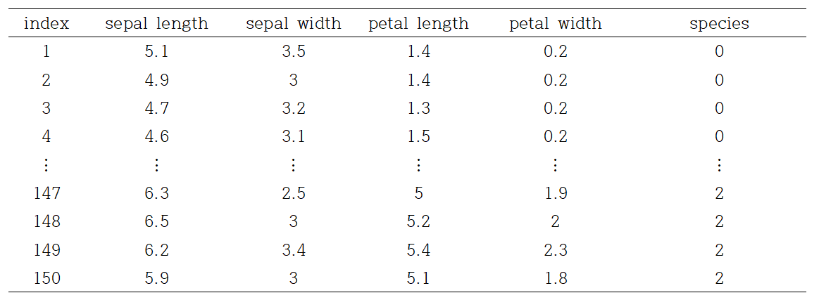
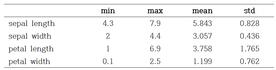
데이터는 사이킷런으로부터 쉽게 사용할 수 있으며, 반응변수를 제외한 모든 설명변수들은 연속형 변수로 구성된다. 데이터 분석의 목적은 꽃의 정보를 이용해 꽃의 종류를 예측하는 것이다. 총 데이터 개수는 150개이다.
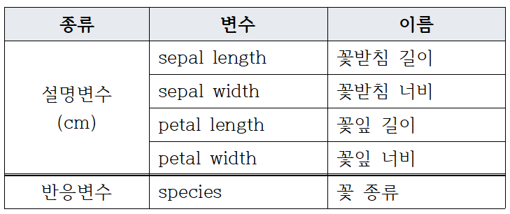
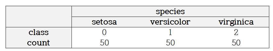
꽃의 종류는 setosa, versicolor, virginica이며, 각 클래스마다 50개의 데이터가 주어진다.
- 변수들의 분포
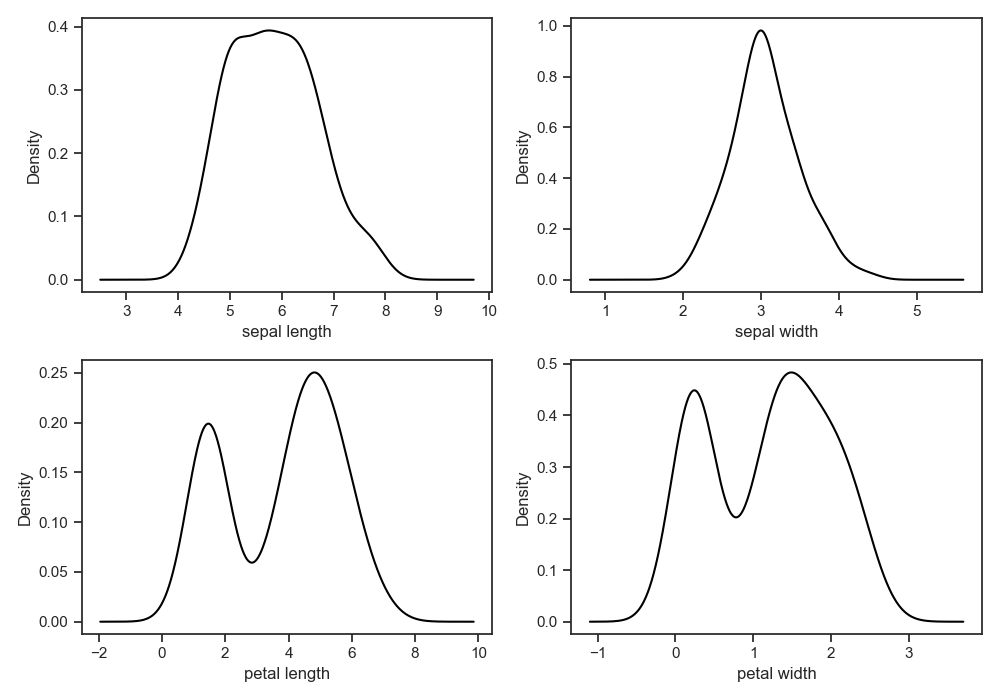
설명변수가 모두 연속형이므로 커널밀도함수를 통해 분포를 확인하였다. 꽃받침 정보 관련한 변수들은 거의 대칭인 분포를 보여준다.
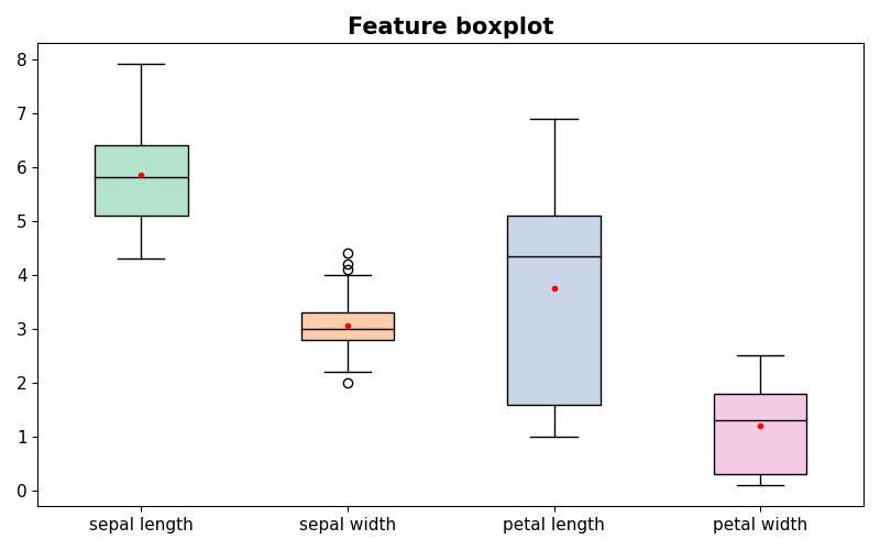
각 변수별 boxplot 분포를 나타낸다. sepal width는 다른 변수들에 비해 이상치가 존재함을 볼 수 있으며, petal width는 다른 변수들에 비해 단위가 작음을 볼 수 있다.
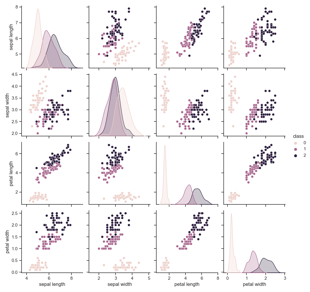
class에 따른 변수들의 분포를 확인하기 위해, pairplot을 생성하였다. 각 클래스마다 서로 다른 색을 가지며, 대각선은 각 클래스마다 해당 변수의 커널밀도추정 그래프를 나타낸다. 꽃 종류 중 setosa는 모든 분포에서 대부분 다른 클래스와 동떨어져 위치해있는 것으로 보아 다른 클래스에 비해 분류하기 쉬울 것으로 예상된다.
그래프 그린 코드 ↓
from sklearn.datasets import load_iris
import pandas as pd
import matplotlib.pyplot as plt

iris = load_iris()

data = pd.DataFrame(iris["data"], columns = iris['feature_names'])
data.loc[:, "species"] = iris["target"]
data.columns = [x.split(" (")[0] for x in data.columns]
data.to_csv("./iris_data.csv", index = False)


'''
데이터 정보
'''

data_info = pd.concat([data.min(), data.max(), data.mean(), data.std()], axis = 1)
data_info.columns = ["Min", "Max", "Mean", "Std"]
data_info.to_csv("./data_info.csv")


'''
박스플랏
'''

colormap = plt.cm.Pastel2

fig,ax = plt.subplots(figsize=(8, 5))
ax, props = data.iloc[:, :-1].boxplot(grid= False, showmeans=True,
                                 meanprops={"marker":"o",
                                           "markerfacecolor":"red",
                                           "markeredgecolor":"red",
                                           "markersize":"3"},
                                 medianprops={"color":"black"},
                                 color = "black", patch_artist=True, return_type='both',
                                 ax = ax)

for i, patch in enumerate(props['boxes']):
        patch.set_facecolor(colormap(i))

plt.title("Feature boxplot", fontsize = 15, fontweight = "bold")
plt.xticks(fontsize = 11)
plt.yticks(fontsize = 11)
plt.tight_layout()


'''
kernel dist
'''

fig, ax = plt.subplots(2, 2, figsize = (10, 7))

k = 0
for i in range(2):
    for j in range(2):
        data.iloc[:, k].plot.kde(ax = ax[i][j], color = "black")
        ax[i][j].set_xlabel(data.columns[k])
        k+=1
plt.tight_layout()


'''
pairplot
'''

import seaborn as sns
sns.set_theme(style="ticks")
sns.pairplot(data, hue = "species")
로지스틱 회귀모델을 생성하기 위해, 손실함수를 최소화하는 방향으로 가중치를 업데이트하는 경사하강법을 적용하고자 한다.
1. 이진분류
주어진 데이터는 3개의 클래스를 갖지만, 단순한 형태의 이진분류를 수행해보기 위해, 다음과 같은 경우를 고려한다.
#1. setosa (0) 종류인가? / 아닌가?
#2. vergicolor (1) 종류인가? / 아닌가?
#3. virginica (2) 종류인가? / 아닌가?
즉, 특정 클래스를 제외한 나머지 클래스 데이터들을 others로 묶어 이진분류의 형태로 변환한다.
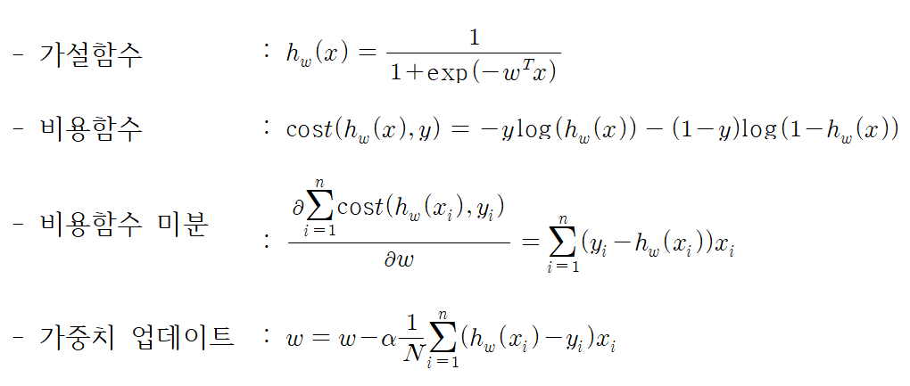
- 로지스틱 회귀분석
우리는 로지스틱 회귀분석 개념 공부를 통해, 가설함수와 비용함수, 비용함수의 미분를 확인했다. 또한, 경사하강법에서 가중치를 업데이트 할 때, 어떤 식을 이용해야 하는지 보았다. 이를 간단하게 짚고 넘어가자.
자세한 설명은 아래 블로그를 참고한다 ↓
https://footprints-toward-data-analysis.tistory.com/7
3. 로지스틱 회귀분석 (Logistic Regression)
우리가 예측하고자 하는 값이 실수, 연속적인 값을 갖는 경우 선형회귀분석을 이용해 이를 설명하는 모델을 탐색한다. 하지만, 만약 우리가 예측하고자 하는 값이 "예/아니오", "10대/20대/30대"와
footprints-toward-data-analysis.tistory.com
3가지 경우를 모두 해보면 좋겠지만, 모두 동일한 작업을 반복하기 때문에 #2. vergicolor (1) 종류인가? / 아닌가? 를 예시로 들고자 한다. 이를 위해 vergicolor인 경우 1로 두고 나머지 꽃의 종류는 0으로 둔다. 즉, vergicolor 종류인 경우 50개의 데이터와 vergicolor가 아닌 나머지 꽃 종류인 경우 100개의 데이터를 이용해 vergicolor를 분류하는 모델을 생성하고자 한다.
이때, 훈련 집합과 테스트 집합은 7:3으로 나누어 구성하였다.
| Train | Test | |
| count | 105 | 45 |
| class (1: vergicolor, 0: other) |
0: 71 1: 34 |
0: 29 1: 16 |
| total | 150 | |
vergicolor 분류 코드 ↓
import numpy as np
import pandas as pd
from sklearn.datasets import load_iris
import matplotlib.pyplot as plt
import seaborn as sns
from sklearn.model_selection import train_test_split

# 로지스틱 함수 정의
def logistic(x):
    return 1/(1+np.exp(-x))

# 비용 함수 정의
def cost(yreal, ypred):
    return np.sum(-yreal*np.log(ypred)-(1-yreal)*np.log(1-ypred))/len(yreal)

# 비용 함수 미분
def cost_diff(yreal, ypred, train_x):
    return np.dot((ypred-yreal), train_x)/len(yreal)

# 최종 predict
def predict(ypred):
    return np.array([0 if x < 0.5 else 1 for x in ypred])


'''
데이터 처리
'''

# 데이터 불러오기
iris = load_iris()

# 분석하기 쉬운 데이터로 변환
data = pd.DataFrame(iris["data"], columns = iris['feature_names'])
data.loc[:, "species"] = iris["target"]
data.columns = [x.split(" (")[0] for x in data.columns]

# 설명변수, 반응변수(3개 클래스) 나누기
X, y = data.iloc[:, :-1].values, data.species


'''
목표
: vergicolor인지 아닌지 분류
'''

# vergicolor 1 나머지 0 (반응변수로 대체)
vergicolor_class = np.where(y == 1, 1, 0)

# train, test 나누기
# 가중치 업데이트를 쉽게 하기 위해 설명변수에 1 추가 (절편 고려)
# train_x, test_x -> grad_train_x, grad_test_x
train_x, test_x, train_y, test_y = train_test_split(X, vergicolor_class, test_size = 0.3, random_state = 0)
grad_train_x, grad_test_x = np.c_[np.ones(len(train_x)), train_x], np.c_[np.ones(len(test_x)), test_x]

# 초기 가중치 랜덤하게 부여
np.random.seed(0)
W = np.random.random(len(grad_train_x[0]))

# 예측값, 비용함수 값 계산
ypred = logistic(np.dot(grad_train_x, W))
prev_cost = cost(train_y, ypred)


'''
GD(경사하강법) 적용
'''

i = 1
alpha = 0.1
while True:

    # 가중치 업데이트
    W = W - alpha * cost_diff(train_y, ypred, grad_train_x)
    ypred = logistic(np.dot(grad_train_x, W))
    next_cost = cost(train_y, ypred)

    if i%50 == 0:
        print("iter:", i)
        print("이전 비용값:", round(prev_cost, 10))
        print("업데이터 후 비용값:", round(next_cost, 10))
        print("b : %.10f, w1 : %.10f, w2 : %.10f, w3 : %.10f, w4 : %.10f" % tuple(W))
        print("-"*50, "\n")

    if abs(prev_cost-next_cost) < 0.1**7:
        break

    prev_cost = next_cost
    i += 1

print("> 총 iteration :", i)
print("  - learning rate :", alpha)
print("  - h(x) = %.3f + (%.3f) sepal length + (%.3f) sepal width + (%.3f) petal length + (%.3f) petal width\n"%tuple(W))

test_ypred_prob = logistic(np.dot(grad_test_x, W))

test_ypred = predict(test_ypred_prob)

print("test 결과")
print("  ---> Logistic Regression 확률: \n", np.round(test_ypred_prob, 3), "\n")
print("  ---> 최종 예측: \n", test_ypred, "\n")


'''
sklearn
'''

from sklearn.linear_model import LogisticRegression

lr = LogisticRegression().fit(train_x, train_y)
sk_ypred = lr.predict(test_x)

sk_W = np.append(lr.intercept_, lr.coef_[0])


print("sklearn test 결과")
print("  - h(x) = %.3f + (%.3f) sepal length + (%.3f) sepal width + (%.3f) petal length + (%.3f) petal width\n"%tuple(sk_W))
print("  ---> 최종 예측: \n", sk_ypred, "\n")
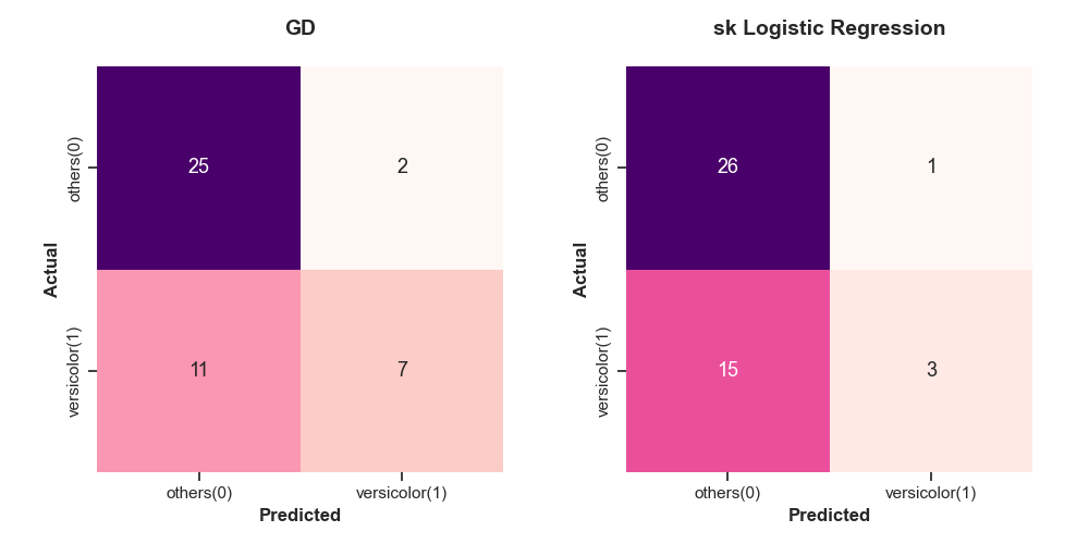
예측 결과는 confusion matrix를 이용해 비교한다. 그 결과, GD는 실제 vergicolor를 제대로 예측한 예제 개수가 7개인 반면, sklearn을 통해 구한 모델은 실제 vergicolor를 제대로 예측한 예제 개수가 3개밖에 되지 않는다. 또한, GD는 13개를 잘못 예측한 반면, sklearn은 16개를 잘못 예측하고 있다. 즉, GD가 sklearn 모델보다 더 좋은 성능을 보인다.
confusion matrix 그린 코드 ↓
from sklearn.metrics import confusion_matrix

fig, ax = plt.subplots(1, 2, figsize = (10, 5))

name = "vergicolor"
cmap = "RdPu"

'''
GD confusion matrix
'''
cm = confusion_matrix(test_y, test_ypred)

ticks = ["others(0)", name+"(1)"] if len(np.unique(test_y)) == 2 else iris.target_names
cmap = color_list[i] if i != 3 else "YlGn"

ax[0].set_title("GD\n", fontsize = 14, fontweight = "bold")
ax[0].set_box_aspect(1)
sns.heatmap(cm, annot=True, cmap=cmap, fmt = "g", cbar=False, annot_kws={"size": 13},
            xticklabels = ticks, yticklabels = ticks,
            ax = ax[0])
ax[0].set_xlabel("Predicted", fontsize = 12, fontweight = "bold")
ax[0].set_ylabel("Actual", fontsize = 12, fontweight = "bold")
plt.tight_layout()


'''
sklearn confusion matrix
'''
sk_cm = confusion_matrix(test_y, sk_ypred)

ax[1].set_title("sk Logistic Regression\n", fontsize = 14, fontweight = "bold")
ax[1].set_box_aspect(1)
sns.heatmap(sk_cm, annot=True, cmap=cmap, fmt = "g", cbar=False, annot_kws={"size": 13},
            xticklabels = ticks, yticklabels = ticks,
            ax = ax[1])
ax[1].set_xlabel("Predicted", fontsize = 12, fontweight = "bold")
ax[1].set_ylabel("Actual", fontsize = 12, fontweight = "bold")

plt.tight_layout()
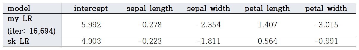
경사하강법을 이용한 로지스틱 회귀모델은 학습률을 0.1로 설정했을 때, 16,694번의 학습을 통해 가중치를 추정했음을 알 수 있다. 각 모델에서 구해진 회귀계수는 서로 다름을 볼 수 있다. sklearn의 Logistic Regression 모델은 최적화 시, "lbfgs"를 사용하여 생성된 모델의 계수 차이가 발생하는 것으로 보인다.
2. 다중분류
이진분류는 경사하강법과 로지스틱 회귀분석을 잘 알면 쉽게 수행할 수 있다.
그렇다면, 로지스틱 회귀분석에서 다중분류는 어떻게 할까?
방법은 각 클래스마다 구한 모델의 예측확률을 이용하는 경우와 소프트맥스 함수를 적용하는 경우가 있다.
이번장에서는 각 클래스마다 구한 모델의 예측확률을 이용하고자 한다. 방법은 매우 쉽다. iris의 경우 #1 ~ #3을 통해 3개의 모델을 생성한다.
#1. setosa (0) 종류인가? / 아닌가?
#2. vergicolor (1) 종류인가? / 아닌가?
#3. virginica (2) 종류인가? / 아닌가?
생성된 3개 모델에 대한 confusion matrix는 다음과 같다.
#1. setosa (0) 종류인가? / 아닌가?
#2. vergicolor (1) 종류인가? / 아닌가?

#3. virginica (2) 종류인가? / 아닌가?
구해진 모델들은 각 예제에 대해서 예측값을 가지고 있다. 이를 이용해 test 집합을 각각 예측한다(train: 70%, test: 30%).
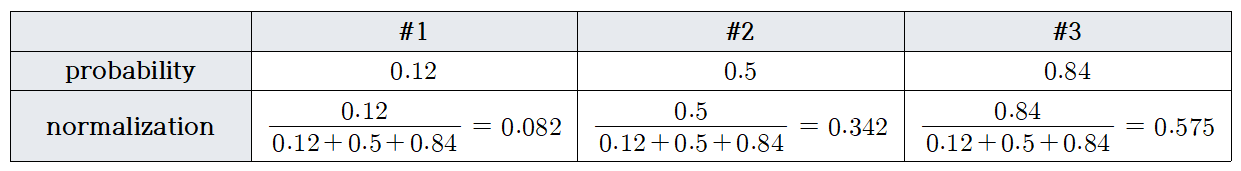
각 test 예제에 대해, 3개의 1일 확률을 얻을 수 있다. 이를 정규화하여, 가장 높은 값을 갖는 클래스로 예측한다.
예를 들어, 테스트 집합 하나에 대해, 각 모델이 0.12, 0.5, 0.84의 확률값을 산출했다고 가정하자. 특정 클래스에 속할 확률을 구하기 위해 정규화하면, #3의 모델의 1일 확률이 가장 높게 측정된다. 그러면 #3의 클래스 1인 virginica로 예측한다.
이를 수행하는 코드는 아래 나타나 있다. 이때, 이전 비용함수 값과 차이가 1e-7 보다 작아지면 루프를 종료하도록 하였다. 더 정확한 모델을 생성하기 위해 1e-7보다 더 작은 값으로 설정하는 경우 오류가 발생한다. 이는 log 계산에서 거의 0의 값을 가져 발생하는 오류로 0이 되지 않도록 매우 작은 값인 1e-16을 더해 계산해준다.
(코드에서는 더해져있음)
import numpy as np
import pandas as pd
from sklearn.datasets import load_iris
import matplotlib.pyplot as plt
import seaborn as sns
from sklearn.model_selection import train_test_split
from sklearn.linear_model import LogisticRegression

# 로지스틱 함수 정의
def logistic(x):
    return 1/(1+np.exp(-x))

# 비용 함수 정의
def cost(yreal, ypred):
    return np.sum(-yreal*np.log(ypred+1e-16)-(1-yreal)*np.log(1-ypred+1e-16))/len(yreal)

# 비용 함수 미분
def cost_diff(yreal, ypred, train_x):
    return np.dot((ypred-yreal), train_x)/len(yreal)

# 최종 predict
def predict(ypred):
    return np.array([0 if x < 0.5 else 1 for x in ypred])


'''
데이터 처리
'''

# 데이터 불러오기
iris = load_iris()

# 분석하기 쉬운 데이터로 변환
data = pd.DataFrame(iris["data"], columns = iris['feature_names'])
data.loc[:, "species"] = iris["target"]
data.columns = [x.split(" (")[0] for x in data.columns]

# 설명변수, 반응변수(3개 클래스) 나누기
# train, test 나누기
X, y = data.iloc[:, :-1].values, data.species.values

train_x, test_x, train_y, test_y = train_test_split(X, y, test_size = 0.3, random_state = 0)


'''
목표
: vergicolor인지 아닌지 분류
'''

# 가중치 업데이트를 쉽게 하기 위해 설명변수에 1 추가 (절편 고려)
# train_x, test_x -> grad_train_x, grad_test_x
grad_train_x, grad_test_x = np.c_[np.ones(len(train_x)), train_x], np.c_[np.ones(len(test_x)), test_x]


'''
경사하강법 적용
'''

info_dic = {"iter":[], "W":[], "pred_prob":[]}

for i in range(3):

    # 특정 클래스 (1), 나머지 (0)
    binary_train_y = np.where(train_y == i, 1, 0)

    # 초기 가중치 랜덤하게 부여
    np.random.seed(0)
    W = np.random.random(len(grad_train_x[0]))

    # 예측값, 비용함수 값 계산
    ypred = logistic(np.dot(grad_train_x, W))
    prev_cost = cost(binary_train_y, ypred)

    iteration = 1
    alpha = 0.1 if i < 2 else 0.8
    while True:

        # 가중치 업데이트
        W = W - alpha * cost_diff(binary_train_y, ypred, grad_train_x)
        ypred = logistic(np.dot(grad_train_x, W))
        next_cost = cost(binary_train_y, ypred)

        if iteration%50 == 0:
            print("iter:", iteration)
            print("이전 비용값:", round(prev_cost, 10))
            print("업데이터 후 비용값:", round(next_cost, 10))
            print("b : %.10f, w1 : %.10f, w2 : %.10f, w3 : %.10f, w4 : %.10f" % tuple(W))
            print("-"*50, "\n")

        if abs(prev_cost-next_cost) < 1e-7:
            binary_test_y = np.where(test_y == i, 1, 0)

            test_ypred_prob = logistic(np.dot(grad_test_x, W))
            test_ypred = predict(test_ypred_prob)

            info_dic["iter"].append(iteration)
            info_dic["W"].append(W)
            info_dic["pred_prob"].append(test_ypred_prob)

            break

        if np.isnan(next_cost):
            break

        prev_cost = next_cost
        iteration += 1


pred_prob_list = np.array(info_dic["pred_prob"])

# 예측확률 정규화
pred_sum = np.sum(pred_prob_list, axis = 0)
pred_prob_final = np.array([x/pred_sum for x in pred_prob_list])

# 예측클래스
final_pred = np.argmax(pred_prob_final, axis = 0)


'''
sklearn
'''

lr = LogisticRegression(max_iter = 5000).fit(train_x, train_y)
sk_ypred = lr.predict(test_x)

sk_W = np.append(lr.intercept_, lr.coef_)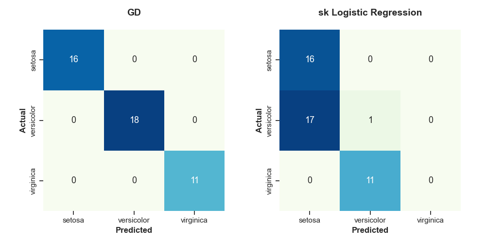
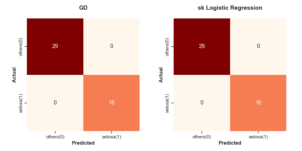
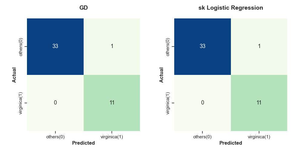
그 결과, 경사하강법으로 수행한 로지스틱 회귀분석이 모든 클래스를 잘 분류함을 볼 수 있다.
오늘은 이전에 배웠던 로지스틱 회귀모델을 경사하강법을 이용하여 생성하였다. 그 결과, 사이킷런 모델의 결과와 비슷하거나 더 나은 결과를 보였다. 다음에는 앙상블 기법인 AdaBoost에 대해서 공부하고자 한다.
'손으로 직접 해보는 모델정리 > 단일 모델' 카테고리의 다른 글
| 7. 의사결정 나무(Decision Tree) (2) | 2023.05.25 |
|---|---|
| 6. KNN: K Nearest Neighbors (0) | 2023.05.12 |
| 4. 경사하강법을 이용한 선형회귀 (0) | 2023.03.08 |
| 3. 로지스틱 회귀분석 (Logistic Regression) (0) | 2023.02.28 |
| 2. 경사하강법 (Gradient Descent) (0) | 2023.01.04 |


